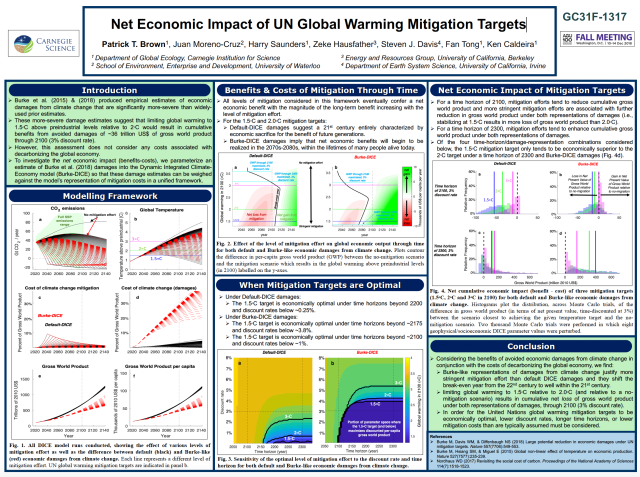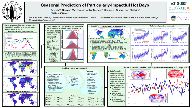
My talk on this research at the American Meteorological Society’s Annual Meeting.

My talk on this research at the American Meteorological Society’s Annual Meeting.
As a climate scientist, I often hear it bemoaned that the public discussion of human-caused global warming is so politically polarized (Pew Research, 2019). The argument goes that global warming is simply a matter of pure science and thus there should be no divisions of opinion along political lines. Since it tends to be the political Right that opposes policies designed to address global warming, the reason for the political division is often placed solely on the ideological stubbornness of the Right.
This is a common theme in research on political divides regarding scientific questions. These divides are often studied from the perspective of researchers on the Left who, rather self-servingly, frame the research question as something like “Our side came to its conclusions from pure reason, so what exactly makes the people who disagree with us so biased and ideologically motivated?” I would put works like The Republican Brain: The Science of Why They Deny Science — and Reality in this category.
Works like The Republican Brain correctly point out that those most dismissive of global warming tend to be on the Right, but they incorrectly assume that the Left’s position is therefore informed by dispassionate logic. If the Left was motivated by pure reason then the Left would not be just as likely as the Right to deny science on the safety of vaccines and genetically modified foods. Additionally, as Mooney has argued elsewhere, the Left is more eager than the Right to deny mainstream science when it doesn’t support a blank-slate view of human nature. This suggests that fidelity to science and logic are not what motivates the Left’s concern about global warming.
Rather than thinking of the political divide on global warming as being the result of logic vs. dogma, a much better explanation is that people tend to accept conclusions, be they scientific or otherwise, that support themes, ideologies, and narratives that are a preexisting component of their worldview (e.g., Washburn and Skitka, 2017). It just so happens that the themes, ideologies, and narratives associated with human-caused global warming and its proposed solutions align well with archetypal worldviews of the Left and create great tension with archetypal worldviews of the Right.
The definitional distinction between the political Right and the political Left originates from the French Revolution and is most fundamentally about the desirability and perceived validity of social hierarchies. Definitionally, those on the Right see hierarchies as natural, meritocratic and justified while those on the Left see hierarchies more as a product of luck and exploitation. A secondary distinction, at least contemporarily in the West, is that those on the Right tend to emphasize individualism at the expense of collectivism and those on the Left prefer the reverse.
There are several aspects of the contemporary human-caused global warming narrative that align well with an anti-hierarchy, collectivist worldview. This makes the issue gratifying to the sensibilities of the Left and offending to the sensibilities of the Right.
The most fundamental of these themes is the degree to which humanity itself can be placed at the top of the hierarchy of life on the planet. Those on the Right would be more likely to articulate that it is justified to privilege the interests of humanity over the interests of other species or the “interests” of the planet as a whole (to the degree that there is such a thing). On the other hand, those on the Left would be more likely to emphasize across-species egalitarianism and advocate for reduced impact on the environment, even if it is against the interest of humans.
Within humanity, there are also at least two levels for which narratives about hierarchies influence thinking on global warming. One is the issue of developed vs. developing countries. The blame for global warming falls disproportionately on developed countries (in terms of historical greenhouse gas emissions) and thus proposed solutions often call on developed countries to bear the brunt of the cost of reducing emissions going forward. (Additionally, it is argued that developed countries have the luxury of being able to afford the associated increases in the cost of energy.) Overall, the solutions proposed for global warming imply that wealthy countries owe a debt to the rest of humanity that should come due sooner rather than later.
Those on the Right are more likely to see the wealth of developed countries as being rightfully earned through their own industriousness while those on the Left are more likely to view the disproportionate wealth of different countries as being fundamentally unjust and likely originating from exploitation. Thus, the story that wealthy countries are to blame for the global warming problem and that the solution is to penalize wealthy countries and subsidize poor countries is one that aligns well with preexisting narratives on the Left but not those on the Right. An accentuating factor is the tendency of the Right to be more in favor of national autonomy and thus opposed to global governance and especially international redistribution.
The third level for which hierarchy narratives couple with political divides on global warming relates to the wealth of corporations and individuals. On the Right, the story of oil and gas companies (as well as electric utilities that utilize fossil fuels) is one of innovation and wealth creation: The smartest and most deserving people and organizations found the most efficient ways to transform idle fossil fuel resources into the power that runs society and greatly enhances human wellbeing. Under such a narrative, it is fundamentally unjust to point a finger of blame at those entities (both corporations and individuals) that have done so much for human progress. The counter-narrative from the Left is that greedy corporations and individuals exploited natural resources for their own gain at the expense of the planet and the general public. Under this narrative, policies that blame and punish those in the fossil fuel industry are seen as bringing about a cosmic justice that is necessary for them to atone for their sins.
The other major overlapping theme that defines the divide between the Left and the Right on global warming is the degree to which collectivism is emphasized compared to individualism. Global warming is fundamentally a tragedy of the commons problem in which logical agents act in such a way that ends up being in the worst interest for everyone in the long term. These types of ‘collective-action problems’ almost necessarily call for top-down government intervention and thus they are inevitably associated with collectivism at the expense of individualism. Also, global warming’s long term nature calls for the embracement of collectivism across generations. Again, this natural alignment of the global warming problem with collectivist themes makes the issue much more palatable for the Left than for the Right.
In addition to these fundamental ideological issues, there are a number of more circumstantial characteristics that’s I believe have contributed to polarization regarding global warming.
One is that, in the U.S. at least, Al Gore was the primary actor that brought global warming into the national consciousness. If one wanted the issue to be “non-political” one couldn’t have conceived of a worse person than a former vice president and presidential nominee to be the main flagbearer for the movement.
Also, there is the longstanding claim by those on the Right that the global warming issue is just a Trojan Horse intended as an excuse to bring about all the desired policies of the Left. Books like This Changes Everything: Capitalism vs. The Climate and plans like the Green New Deal do little to dispel this narrative. For example, the Green New Deal Resolution contained the following proposals:
“Providing all people of the United States with— (i) high-quality health care; (ii) affordable, safe, and adequate housing; (iii) economic security; and (iv) access to clean water, clean air, healthy and affordable food, and nature.”
“Guaranteeing a job with a family-sustaining wage, adequate family and medical leave, paid vacations, and retirement security to all people of the United States.”
“Providing resources, training, and high-quality education, including higher education, to all people of the United States, with a focus on frontline and vulnerable communities, so those communities may be full and equal participants in the Green New Deal mobilization”.
These are objectives that clearly seek to satisfy goals of the Left but it is much less clear how directly related these objectives are to global warming.
So, it should really not be particularly mysterious that opinions on global warming tend to divide along political lines. It is not because one side embraces pure reason while the other remains obstinately wedded to political dogmatism. It is simply that the problem and its proposed solutions align more comfortably with the dogma of one side than the other. That does not mean, however, that the Left is equally out-of-step with the science of global warming as the Right. It really is the case that the Right is more likely to deny the most well-established aspects of the science. But, if skeptical conservatives are to be convinced, the Left must learn to reframe the issue in a way that is more palatable to their worldview.
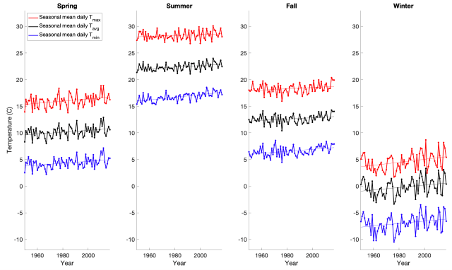
The graph above is a record of temperature from 1950-2017 for New York City.
What is unique about this graph is that it shows daily, seasonal, annual and decadal temperature variability on a single Y-axis, revealing how their magnitudes compare.
The daily temperature cycle is represented by the three colored lines in each panel, where red, black and blue represent the daily maximum, daily average and daily minimum for each season and year. For example, the red dots in the far left panel represent the average of all the daily maximum temperatures for the spring of each year.
We can see that in New York, the daily minimum temperature tends to be around 13 degrees C (23 degrees F) lower than the daily maximum temperature.
The annual temperature cycle is illustrated by the variation across the four panels with each panel representing one of the four canonical seasons.
We can see that in New York, the summer tends to be about 22 degrees C (40 degrees F) warmer than the winter.
Interannual temperature variability is illustrated by the year-to-year wiggles in each line.
We can see that in New York, there can be year-to-year swings in temperature (for a given season) of several degrees C. For example, the summer of 1999 had a daily average temperature of 24 C (75 F) and the summer of 2000 had a daily average temperature of 21 C (70 F). It is also notable that year-to-year variability in winter temperature is substantially larger than year-to-year variability in summer temperature.
Decadal temperature changes are represented by the linear trend lines. We can see long term warming which is primarily driven by increases in greenhouse gasses (i.e., this is the local manifestation of global warming). The long term warming is generally more prominent in the daily minimum temperature compared to the daily maximum temperature and more prominent in the winter compared to the summer. In other words, global warming is shrinking both the daily and seasonal temperature cycles.
In terms of absolute magnitude, the seasonal cycle is the dominant mode of variability, followed by the daily cycle, year-to-year variability and finally, long term warming.
Thus, while Global Warming is very pronounced on global spatial scales and centennial and greater timescales, we can see that, thus far, it has had a modest influence on the temperature in New York relative to the typical variability at the daily, seasonal and annual timescales.
Data here is from Berkeley Earth.
The El-Niño Southern Oscillation (ENSO) is the preeminent mode of global climate variability on timescales of months to several years. El Niño events cause temporary elevations in global average temperatures, and in the context of background global warming from increasing greenhouse gas concentrations, El Niño events are often associated with setting new global temperature records. El Niños cause warmer than typical global average temperatures because they are associated with a great amount of heat release from the equatorial Pacific to the atmosphere which is then distributed globally. This release of heat also imprints on the structure of the atmosphere and shifts the tendencies of typical atmospheric circulations. In certain locations, advection from climatologically colder locations (e.g., flow from the north in the Northern Hemisphere) becomes more prominent than normal during El Niño events which can cause a local tendency for temperatures to cool during El Niños, despite elevated temperatures globally. The large scale atmospheric circulation is also influenced by the state of ENSO differently depending on the time of the year.
This all means that if you want to translate the state of ENSO into a seasonal forecast (e.g., a forecast for 3-month average temperatures) at a particular location, you have to be careful to examine both the specific relationship between ENSO and climate variability at the location you are interested in as well as how that relationship depends on the time of the year. This is the purpose of the Simple ENSO Regression Forecast (SERF).
The SERF is based on an ensemble of dynamical and statistical model forecasts that predict the future state of ENSO, combined with the historical relationships between the state of ENSO and concurrent local surface air temperature departures from average (as a function of location and time of the year).
At ClimateAi, we are developing considerably more sophisticated machine learning techniques for application to seasonal forecasting that are able to achieve enhanced skill over this simple method. Nevertheless, this simple method is transparent and serves as a useful benchmark for more sophisticated methods to be compared to.
Below is the Simple ENSO Regression Forecast (SERF) for the 2019 Northern Hemisphere summer and Southern Hemisphere winter (June-July-August 2019). A weak El-Niño like state is expected to persist throughout the upcoming season. This translates into an expectation for below normal temperatures over northern/central Canada, the US upper Midwest and much of Russia. Above average temperatures are expected over the US Pacific Northwest, Mexico, much of South America, Africa, India, the Middle East and Europe (see Figure 1 and Figure 2 below). One reason that the tropics shows more consistent warming is that the background global warming has a higher signal-to-noise ratio there which means it is more likely that any given season will be above its 1971-2000 average, regardless of the state of ENSO.
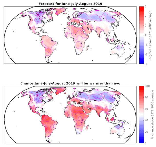
Figure 1. Top) SERF forecast of the average temperature for June-July-August 2019 relative to the long term average (from 1971-2000) for each location. Bottom) Chance that the average temperature over June-July-August will be above the long term average (from 1971-2000) for June-July-August at that location.
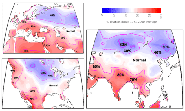
Figure 2. Same as the bottom of figure 1 but zoomed in to particular regions.
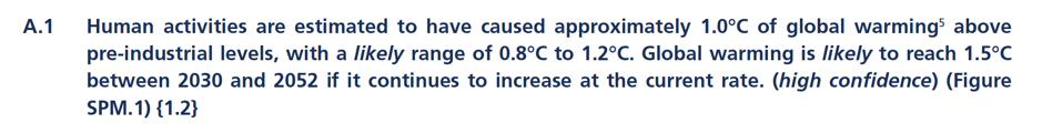
In late 2018 the Intergovernmental Panel on Climate Change (IPCC) released a report on the impacts associated with global warming of 1.5°C (2.7°F) above preindustrial levels (as of 2019 we are at about 1.0°C above pre-industrial levels) as well as the technical feasibility of limiting global warming to such a level. The media coverage of the report immediately produced a meme that continues to persist. The meme is some kind of variation of the following:
The IPCC concluded that we have until 2030 (or 12 years) to avoid catastrophic global warming
Below is a sampling of headlines from coverage that propagated this meme.
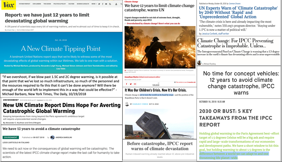
However, these headlines are essentially purveying a myth. I think it is necessary to push back against this meme for two main reasons:
1) It is false.
2) I believe that spreading this messaging will ultimately undermine the credibility of the IPCC and climate science more generally.
Taking these two points in turn:
1) The IPCC did not conclude that society has until 2030 to avoid catastrophic global warming.
First of all, the word “catastrophic” does not appear in the IPCC report. This is because the report was not tasked with defining a level of global warming which might be considered to be catastrophic (or any other alarming adjective). Rather, the report was tasked with evaluating the impacts of global warming of 1.5°C (2.7°F) above preindustrial levels, and comparing these to the impacts associated with 2.0°C (3.6°F) above preindustrial levels as well as evaluating the changes to global energy systems that would be necessary in order to limit global warming to 1.5°C.
In the report, the UN has taken the strategy of defining temperature targets and then evaluating the impacts at these targets rather than asking what temperature level might be considered to be catastrophic. This is presumably because the definition of a catastrophe will inevitably vary from country to country and person to person, and there is not robust evidence that there is some kind of universal temperature threshold where a wide range of impacts suddenly become greatly magnified. Instead, impacts seem to be on a continuum where they simply get worse with more warming.
So what did the IPCC conclude regarding the impacts of global warming of 1.5°C? The full IPCC report constituted an exhaustive literature review but the main conclusions were boiled down in the relatively concise summary for policymakers. There were six high-level impact-related conclusions:
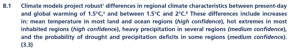
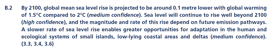

So to summarize the summary, the IPCC’s literature review found that impacts of global warming at 2.0°C are worse than at 1.5°C.
The differences in tone between the conclusions of the actual report and the media headlines highlighted above are rather remarkable. But can some of these impacts be considered to be catastrophic even if the IPCC doesn’t use alarming language? Again, this would depend entirely on the definition of the word catastrophic.
If one defines catastrophic as a substantial decline in the extent of artic sea ice, then global warming was already catastrophic a couple decades ago. If global warming intensified a wild fire to the extent that it engulfed your home (whereas it would not have without global warming) then global warming has already been catastrophic for you.
However, I do not believe that changes in arctic sea ice extent and marginal changes in damages from forest fires (or droughts, floods etc.) are what most people envision when they think of the word catastrophic in this context. I believe that the imagery evoked in most peoples’ minds is much more at the scale of a global apocalyptic event. This idea is exemplified in Michael Barbaro’s question about the IPCC report that he asked on The New York Times’ The Daily:
“If we overshoot, if we blow past 1.5°C and 2°C degree warming, is it possible at that point that we’ve lost so much infrastructure, so much of the personnel and the resources required to fix this that it can’t be done anymore? Will there be enough of the world left to implement this in a way that could be effective?”
-Michael Barbaro, New York Times, The Daily, 10/19/2018
It is also articulated in a tweet from prominent climate science communicator Eric Holthaus:
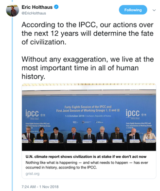
If catastrophe is defined as global-scale devastation to human society then I do not see how it could be possible to read the IPCC report and interpret it as predicting catastrophe at 1.5°C or 2°C of warming. It simply makes no projections approaching such a level of alarm.
2. Undermining credibility.
Some will object to me pointing out that the IPCC has not predicted a global-scale societal catastrophe by 2030. They will inevitably suggest that whether or not the meme is strictly true, it is useful for motivating action on climate policy and therefore it is counterproductive to push back against it. I could not disagree more with this line of thinking.
The point of a document like the IPCC report should be to inform the public and policy makers in a dispassionate and objective way, not to make a case in order to inspire action. The fundamental reason for trusting science in general (and the IPCC in particular) is the notion that the enterprise will be objectively evaluating our best understanding of reality, not arguing for a predetermined outcome. I believe that the IPCC report has adhered to the best scientific standards but the meme of a predicted catastrophe makes it seem as though it has veered into full advocacy mode – making it appear untrustworthy.
An on-the-record prediction that may come back to haunt us
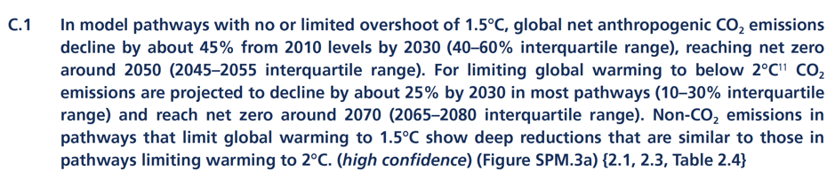
Apart from the inaccurate characterization that the IPCC has projected a catastrophe at 1.5°C, the other potentially harmful aspect of the media headlines above is that they put a timetable on the catastrophe that is very much in the near-term (2030). The year 2030 comes from the idea that we could first cross the 1.5°C threshold (at the annual mean level) in 2030, as is articulated in the report:
Now, if we immediately implement the global climate policies necessary to avoid 1.5°C of warming, then the prediction of a catastrophe will never be put to the test. However, as the IPCC report makes clear, achieving the cuts in emissions necessary to limit global warming to 1.5°C represents a truly massive effort:

Given that this effort would likely be massively expensive and represents a large technical challenge, it is unlikely to occur. This means that we are likely to pass 1.5°C of warming sometime in the 2030s, 2040s or 2050s. At this point – assuming that nothing resembling what most people would consider to be a global societal catastrophe has occurred – the catastrophe meme associated with the 2018 IPCC report will be dredged up and used as ammunition against the credibility of climate science and the IPCC. I fear that it will be used to undermine any further scientific evaluation of impacts from global warming.
In my experience, the primary reason that people skeptical of climate science come to their skepticism is that they believe climate scientists are acting as advocates rather than dispassionate evaluators of evidence. They believe climate scientists are acting as lawyers, making the case for climate action, rather than judges objectively weighing facts. The meme of a global catastrophe by 2030 seems to put a prediction on the record that is likely to be proven false and thus likely to reinforce this notion of ‘climate scientists as untrustworthy activists’ and thus harm the credibility of climate science thereafter.
This autumn has been very dry in California and this has undoubtedly increased the chance of occurrence of the deadly wildfires that the state is seeing.
When assessing the influence of global warming (from human burning of fossil fuels) on these fires, it is relevant to look at climate model projections of extremely dry autumn conditions in California. Below is an animation that uses climate models to calculate the odds that any given November in California will be extremely dry.
Here, extremely dry is defined as a California statewide November that is characterized by soil moisture content three standard deviations below the mean, where the mean and standard deviation is defined over the period 1860-1900.
We can see that these extremely dry Novembers in California go from being exceptionally rare early in the period (by definition), to being more likely now (~1% chance), and much more likely by the end of the century (~7% chance).
In terms of an odds ratio, this would indicate that “extremely dry” conditions are approximately 7 times more likely now than they were at the end of the 19th century and that these “extremely dry” conditions would be approximately 50 times more likely at the end of the century under an RCP8.5 scenario.
*chance is calculated by looking at the frequency of California Novembers below the 3 standard deviation threshold across all CMIP5 ensemble members (70) and using a moving window of 40 years.
Nature has published a Brief Communications Arising between us (Patrick Brown, Martin Stolpe, and Ken Caldeira) and Peter Cox, Femke Nijsse, Mark Williamson and Chris Huntingford; which is in regards to their paper published earlier this year titled “Emergent constraint on equilibrium climate sensitivity from global temperature variability” (Cox et al. 2018).
Summary
Background
The Cox et al. (2018) paper is about reducing uncertainty in the amount of warming that we should expect the earth to experience for a given change in greenhouse gasses. Their abstract gives a nice background and summary of their findings:
Equilibrium climate sensitivity (ECS) remains one of the most important unknowns in climate change science. ECS is defined as the global mean warming that would occur if the atmospheric carbon dioxide (CO2) concentration were instantly doubled and the climate were then brought to equilibrium with that new level of CO2. Despite its rather idealized definition, ECS has continuing relevance for international climate change agreements, which are often framed in terms of stabilization of global warming relative to the pre-industrial climate. However, the ‘likely’ range of ECS as stated by the Intergovernmental Panel on Climate Change (IPCC) has remained at 1.5–4.5 degrees Celsius for more than 25 years. The possibility of a value of ECS towards the upper end of this range reduces the feasibility of avoiding 2 degrees Celsius of global warming, as required by the Paris Agreement. Here we present a new emergent constraint on ECS that yields a central estimate of 2.8 degrees Celsius with 66 per cent confidence limits (equivalent to the IPCC ‘likely’ range) of 2.2–3.4 degrees Celsius.
Thus, the Cox et al. (2018) study found a (slight) reduction in the central estimate of climate sensitivity (2.8ºC relative to the oft-quoted central estimate of 3.0ºC) and a large reduction in the uncertainty for climate sensitivity, as they state in their press release on the paper:
While the standard ‘likely’ range of climate sensitivity has remained at 1.5-4.5ºC for the last 25 years the new study, published in leading scientific journal Nature, has reduced this range by around 60%.
Combining these two results drastically reduces the likelihood of high values of climate sensitivity. This finding was highlighted by much of the news coverage of the paper. For example, here’s the beginning of The Guardian’s story on the paper:
Earth’s surface will almost certainly not warm up four or five degrees Celsius by 2100, according to a study which, if correct, voids worst-case UN climate change predictions.
A revised calculation of how greenhouse gases drive up the planet’s temperature reduces the range of possible end-of-century outcomes by more than half, researchers said in the report, published in the journal Nature.
“Our study all but rules out very low and very high climate sensitivities,” said lead author Peter Cox, a professor at the University of Exeter.
Our Comment
I was very interested in the results of Cox et al. (2018) for a couple of reasons.
First, just a few weeks prior to the release of Cox et al. (2018) we had published a paper (coincidentally, also in Nature) which used a similar methodology but produced a different result (our study found evidence for climate sensitivity being on the higher end of the canonical range).
Second, the Cox et al. (2018) study is based on an area of research that I had some experience in: the relationship between short-term temperature variability and long-term climate sensitivity. The general idea that these two things should be related has been around for a while (for example, it’s covered in some depth in Gerard Roe’s 2009 review on climate sensitivity). But in 2015 Kevin Bowman suggested to me that “Fluctuation-Dissipation Theorem” might be useful for using short-term temperature variability to narrow uncertainty in climate sensitivity. It just so happens that this is the same theoretical foundation that underlies the Cox et al. (2018) results. Following Bowman’s suggestion, I spent several months looking for a useful relationship but I was unable to find one.
Thus, when Cox et al. (2018) was published, I was naturally curious about the specifics of how they arrived at their conclusions both because their results diverged from that of our related study and because they used a particular theoretical underpinning that I had previously found to be ineffectual.
I worked with Martin Stolpe and Ken Caldeira to investigate the Cox et al. (2018) methodology in some detail and to conduct a number of sensitivity tests of their results. We felt that our experiments pointed to some issues with aspects of the study’s methodology and that lead us to submit the aforementioned comment to Nature.
In our comment, we raise two primary concerns.
First, we point out that most of the reported 60% reduction in climate sensitivity uncertainty originates not from the constraint itself but from the choice of the baseline that the revised uncertainty range is compared to. Specifically, the large reduction in uncertainty depends on their choice to compare their constrained uncertainty to the broad IPCC ‘likely’ range of 1.5ºC-4.5ºC rather than to the ‘likely’ range of the raw climate models used to inform the analysis. This choice would be justifiable if the climate models sampled the entire uncertainty range for climate sensitivity but this is not the case. The model ensemble happens to start with an uncertainty range that is about 45% smaller than the IPCC-suggested ‘true’ uncertainty range (which incorporates additional information from e.g., paleoclimate studies). Since the model ensemble embodies a smaller uncertainty range than the IPCC range, one could simply take the raw models, calculate the likely range of climate sensitivity using those models, and claim that this calculation alone “reduces” climate sensitivity uncertainty by about 45%. We contend that such a calculation would not tell us anything meaningful about true climate sensitivity. Instead, it would simply tell us that the current suite of climate models don’t adequately represent the full range of climate sensitivity uncertainty.
Thus, even if the other methodological choices of Cox et al. (2018) are accepted as is, close to 3/4ths of the reported 60% reduction in climate sensitivity uncertainty is attributable to starting from a situation in which the model ensemble samples only a fraction of the full uncertainty range in climate sensitivity.
The second issue that we raise has to do with the theoretical underpinnings of the Cox et al. (2018) constraint. Specifically, The emergent constraint presented by Cox et al. (2018), based on the Fluctuation-Dissipation Theorem, “relates the mean response to impulsive external forcing of a dynamical system to its natural unforced variability” (Leith, 1975).
In this context, climate sensitivity represents the mean response to external forcing, and the measure of variability should be applied to unforced (or internally generated) temperature variability. Cox et al. (2018) state that their constraint is founded on the premise that persistent non-random forcing has been removed:
If trends arising from net radiative forcing and ocean heat uptake can be successfully removed, the net radiative forcing term Q can be approximated by white noise. Under these circumstances, equation (1) … has standard solutions … for the lag-one-year autocorrelation of the temperature.
They suggest that linear detrending with a 55-year moving window may be optimal for the separation of forced trends from variability:
Figure 4a shows the best estimate and 66% confidence limits on ECS as a function of the width of the de-trending window. Our best estimate is relatively insensitive to the chosen window width, but the 66% confidence limits show a greater sensitivity, with the minimum in uncertainty at a window width of about 55 yr (as used in the analysis above). As Extended Data Fig. 3 shows, at this optimum window width the best-fit gradient of the emergent relationship between ECS and Ψ (= 12.1) is also very close to our theory-predicted value of 2 Q2×CO2/σQ (= 12.2). This might be expected if this window length optimally separates forced trend from variability.
Linearly detrending within a moving window is an unconventional way to separate forced from unforced variability and we argue in our comment that it is inadequate for this purpose. (In their reply to our comment Cox et al. agree with this but they contend that mixing forced and unforced variability does not present the problem that we claim it does.)
Using more conventional methods to remove forced variability, we find that the Cox et al. (2018) constraint produces central estimates of climate sensitivity that lack a consistent sign shift relative to their starting value (i.e., it is not clear if the constraint shifts the best estimate of climate sensitivity in the positive or negative direction).
We also find that the more complete removal of forced variability produces constrained confidence intervals on climate sensitivity that range from being no smaller than the raw model confidence intervals used to inform the analysis (Fig. 1d and 1e) to being about 11% smaller than the raw model range (Fig. 1f). This is compared to the 60% reduction in the size of the confidence interval reported in Cox et al., (2018).

Figure 1 | Comparison of central estimate and ‘likely’ range (>66%) of Equilibrium climate sensitivity over a variety of methodologies and for four observational datasets. Average changes (across the four observational datasets) in the central estimates of climate sensitivity are reported within the dashed-line range, average changes in uncertainty ranges (confidence intervals) are reported at the bottom of the figure, and r2 values of the relationship are reported at the top of the figure. Results corresponding to observations from GISTEMP, HadCRUT4, NOAA and Berkeley Earth are shown in black, red, blue and green respectively. Changes in uncertainty are reported relative to the raw model range (±0.95 standard deviations across the climate sensitivity range of CMIP5 models) used to inform the analysis (b) rather than relative to the broader IPCC range used as the baseline in Cox et al. (2018) (a).
Overall, we argue that historical temperature variability provides, at best, a weak constraint on climate sensitivity and that it is not clear if it suggests a higher or lower central estimate of climate sensitivity relative to the canonical 3ºC value.
For more details please see the original Cox et al. (2018) paper, our full comment and the reply to our comment by Cox et al.
Human-caused climate change from increasing greenhouse gasses is expected to influence many weather phenomena including extreme events. However, there is not yet a detectable long-term change in many of these extreme events, as is recently emphasized by Roger Pielke Jr. in The Rightful Place of Science: Disasters and Climate Change.
This means that we have a situation where there is no detectable long-term change in e.g., tropical cyclone heavy rainfall and yet we have studies that conclude that human-caused climate change made Hurricane Harvey’s rainfall 15% heavier than it would have been otherwise. This is not actually a contradiction and the video below shows why.