1) What is a climate model?

In order to correctly interpret climate model output it is important to first understand what a computer climate model is. Climate models are software that simulate the whole earth system by using our knowledge of physics at smaller spatial scales. Climate models break the entire earth into three-dimensional cubes (or grid boxes) and thousands of physical equations are used to simulate the state of each grid box as a function of time (Figure 1).

Because climate models are based on physics (as opposed to the statistics of past events), they can be used to make predictions that have no analogs in the historical record. For example, you could ask the question: “What would India’s climate be like if Africa didn’t exist?” Obviously you can’t use historical statistics to answer such a question but a climate model can make a reasonable prediction based on physics. Similarly, when a climate model projects the climate of 2100 under enhanced greenhouse gas concentrations, it is basing this projection on physics and not any historical analog.

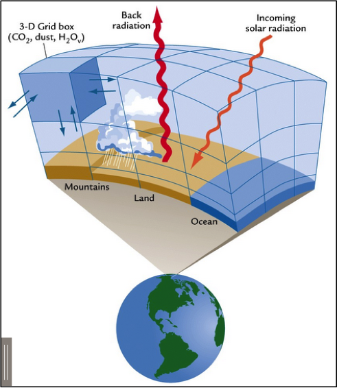
Figure 1. Illustration of the three-dimensional grid of a climate model (from Ruddiman, 2000)

2) Future Climate Change Projections Based on Greenhouse Gas Scenarios

 Climate models are the primary tools used to project changes in the earth system under enhanced greenhouse gas concentrations. Climate models take information about greenhouse gas emissions or concentrations as an input and then simulate the earth system based on these numbers.

3) How greenhouse gas scenarios are input into the models

For CO₂, a climate model that features a fully coupled “carbon cycle model” will only require anthropogenic emissions of CO₂ as an input and it will predict the atmospheric concentrations of CO₂. If a climate model does not have an embedded carbon cycle model, it will require atmospheric concentrations of CO₂ as an input variable. The emissions and concentrations that are used as inputs to the model can be whatever the user desires.

4) Representation of greenhouse gasses in climate models

The most consequential effect of CO₂ in a climate model is that it interacts differently with incoming shortwave radiation than it does with outgoing longwave radiation (this is essentially the definition of a greenhouse gas). The climate model keeps track of radiation in every atmospheric grid box (Figure 1) and at every time step. This is the primary way in which a change in greenhouse gasses will affect the climate of the model. As an example, if you double CO₂ concentrations in a climate model, that model might predict that average rainfall intensity will increase over some arbitrary region. However, the only direct effect of changing CO₂ concentration was that it changed outgoing longwave radiation. Any other change that the model simulates, e.g., the change in rainfall intensity, was secondary and came about due a series of physical links. These links are not necessarily obvious and many scientists spend their careers trying to figure them out.

5) Weather vs. Climate.

Climate is often colloquially defined as “average weather”. Therefore, in order to know the climate at a given location, you generally need weather records over a long period of time (usually 30 years or more). Weather is random and difficult to predict (it is nearly impossible to know if it will rain in New York on July 17th 2015). Climate, on the other hand, is relatively predictable (New York should expect about 120 mm of rain per July on average).

It is important to understand that climate models do not actually simulate climate. Instead, climate models simulate weather. For example, if you run a climate model from the year 2000 to the year 2100 (incorporating an estimated increase in greenhouse gas concentrations) the climate model will simulate the weather over the entire surface of the earth and output its calculations every three hours or so for 100 years. Therefore, the climate model will simulate the weather in New York on July 17th 2088. However, because weather is so unpredictable, nobody should take this “weather forecast” seriously. What may be taken seriously, however, are the long-term trends in July precipitation in New York over the entire course of the simulation.

6) How to interpret climate model output

Imagine that we have climate model output for some climate variable (at a given location) over the next 100 years under a scenario of increasing greenhouse gas concentrations (Figure 2A). We notice that the variable increases and peaks during “Time period A” and then decreases until “Time period B”. We want to know if this pattern is part of the climate change signal (i.e., did the increase in greenhouse gasses cause this pattern?) or if it is just the result of random weather noise. The only way to find out is to run the climate model again (allowing it to simulate different random weather) and see if the same pattern shows up again.

Figure 2B shows output from a 2nd climate model run which incorporated the same increase in greenhouse gas concentrations as the 1^st. We see that, in this case, the variable is higher over “Time period B” than it was over “Time period A”. This indicates that the pattern we saw in the first run may have just been due to random weather noise and not a part of the climate change signal that we are most interested in. To be sure, we can look at a large number of different climate model runs that incorporate the same increase in greenhouse gas concentrations (Figure 2C). It becomes apparent that the common attribute between the runs is a long-term upward trend. If we have enough runs we can average them together to get an estimate of what the true climate change signal is (Figure 2D). Climate is the average weather so averaging over all of the models (taking the “multi-model-mean”) should leave only the portion of the change that is due to the increased greenhouse gas concentrations.

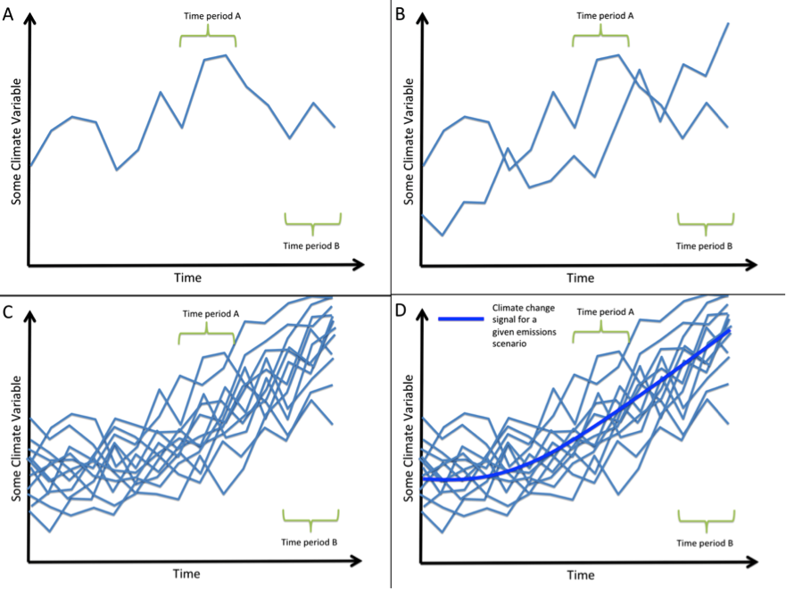
Figure 2. Illustration of the difference between the random weather produced by a single climate model run and the climate change signal that can only be seen when multiple climate model runs are averaged together.

7) Comparing the output of two different scenarios with different greenhouse increases

Figure 3A illustrates a hypothetical comparison of climate model output under two different greenhouse gas emissions scenarios. It would be difficult to interpret the results if we only had a single climate model run from each scenario because we might happen see a progression that is not representative of the underlying climate change signal. For example, it would be possible to see a green run that showed a larger increase in the variable than a blue run even though their respective climate change signals indicate the reverse. In order to compare the climate change signals between the two scenarios we need to average over a number of runs (Figure 3B). It is then possible to use the average and the spread about the average to test whether or not the difference in the emissions scenarios had a meaningful effect on the output variable at some time in the future.

Figure 3. Illustration of climate model output for two different emissions scenarios (blue and green) 

8) Issues to keep in mind when interpreting climate model output

1. Signal to noise ratio may be very small

For many variables, the underlying climate change signal (thick lines in Figures 2 and 3B) may change only a tiny amount relative to how large the variations of the random weather noise is. This means that when we compare the multi-model-mean from one greenhouse gas emissions scenario to another, the difference we see may be due almost entirely to random weather noise instead of being due to some climate change signal.

2. Climate change in the real world will not follow the smooth signal

There is random weather in the real climate system, just like there is in the individual climate model runs. So the true evolution of a variable in the future will not look like the smooth signal. Instead it will look like one of the individual erratic runs. This means that there is a very wide range of values that could be plausible for any given time in the future.

3. It is difficult to validate climate models

Weather is unpredictable and thus we do not expect climate models to be able to reproduce the random weather that has occurred historically. Instead we expect climate models to be able to reproduce the underlying climate change signal that has occurred historically. Unfortunately, our observations over the past 50 to 100 years contain both random weather and a climate change signal but we don’t necessarily know which one is which.

For example, lets say that we observe an increase in drought at some location over the past 20 years. Then we run a set of climate models with historical increases in greenhouse gas concentrations and we see that the models do not suggest that there should have been an increase in drought in this location. This could mean one of two things: 1) the models are deficient and need to be improved before they can simulate this increase in drought or 2) the models are correct and the observed increase in drought was just due to random weather. It is very difficult to know which is the case and that makes it very difficult to assess how well the models are doing.

Since it is so hard to validate the climate models, it is difficult to know how confident we should be in their projections. Nevertheless their output is taken seriously because it probably represents our best quantitative estimate of the future based on our current knowledge of the physical workings of the climate system.

4. Climate models are better at simulating larger spatial/temporal scales than smaller spatial/temporal scales

One problem with climate models is that their spatial and temporal resolution is too coarse to simulate many aspects of the climate that are relevant to society. For example, tornadoes are much smaller than the spatial grid (Figure 1) and much more short-lived than the time step (~3 hours) of a climate model so they cannot possibly be simulated. Even events such as floods tend to be caused by thunderstorms that are smaller-scale than the typical model’s resolution and thus it is difficult for models to correctly simulate the statistics of flooding events.